Lanczos algorithm

Lanczos algorithm

From Wikipedia, the free encyclopedia
The Lanczos algorithm is an iterative algorithm invented by Cornelius Lanczos that is an adaptation of power methods to findeigenvalues and eigenvectors of a square matrix or the singular value decomposition of a rectangular matrix. It is particularly useful for finding decompositions of very large sparse matrices. In Latent Semantic Indexing, for instance, matrices relating millions of documents to hundreds of thousands of terms must be reduced to singular-value form.
Peter Montgomery published in 1995 an algorithm, based on the Lanczos algorithm, for finding elements of the nullspace of a large sparse matrix over GF(2); since the set of people interested in large sparse matrices over finite fields and the set of people interested in large eigenvalue problems scarcely overlap, this is often also called the block Lanczos algorithm without causing unreasonable confusion. See Block Lanczos algorithm for nullspace of a matrix over a finite field.

Inverse iteration

Inverse iteration

From Wikipedia, the free encyclopedia
In numerical analysisinverse iteration is an iterative eigenvalue algorithm. It allows to find an approximate eigenvector when an approximation to a corresponding eigenvalue is already known. The method is conceptually similar to the power method and is also known as the inverse power method.

Rayleigh quotient iteration

Rayleigh quotient iteration

From Wikipedia, the free encyclopedia
Rayleigh quotient iteration is an eigenvalue algorithm which extends the idea of the inverse iteration by using the Rayleigh quotient to obtain increasingly accurate eigenvalue estimates.
Rayleigh quotient iteration is an iterative method, that is, it must be repeated until it converges to an answer (this is true for all eigenvalue algorithms). Fortunately, very rapid convergence is guaranteed and no more than a few iterations are needed in practice. The Rayleigh quotient iteration algorithm converges cubically, given an initial vector that is sufficiently close to an eigenvector of thematrix that is being analyzed.

Power iteration

Power iteration

From Wikipedia, the free encyclopedia
In mathematics, the power iteration is an eigenvalue algorithm: given a matrix A, the algorithm will produce a number λ (theeigenvalue) and a nonzero vector v (the eigenvector), such that Av = λv.
The power iteration is a very simple algorithm. It does not compute a matrix decomposition, and hence it can be used when A is a very large sparse matrix. However, it will find only one eigenvalue (the one with the greatest absolute value) and it may converge only slowly.

Lanczos algorithm

Lanczos algorithm

From Wikipedia, the free encyclopedia
The Lanczos algorithm is an iterative algorithm invented by Cornelius Lanczos that is an adaptation of power methods to findeigenvalues and eigenvectors of a square matrix or the singular value decomposition of a rectangular matrix. It is particularly useful for finding decompositions of very large sparse matrices. In Latent Semantic Indexing, for instance, matrices relating millions of documents to hundreds of thousands of terms must be reduced to singular-value form.
Peter Montgomery published in 1995 an algorithm, based on the Lanczos algorithm, for finding elements of the nullspace of a large sparse matrix over GF(2); since the set of people interested in large sparse matrices over finite fields and the set of people interested in large eigenvalue problems scarcely overlap, this is often also called the block Lanczos algorithm without causing unreasonable confusion. See Block Lanczos algorithm for nullspace of a matrix over a finite field.
Arnoldi iteration

Arnoldi iteration

From Wikipedia, the free encyclopedia
In numerical linear algebra, the Arnoldi iteration is an eigenvalue algorithm and an important example of iterative methods. Arnoldi finds the eigenvalues of general (possibly non-Hermitianmatrices; an analogous method for Hermitian matrices is the Lanczos iteration. The Arnoldi iteration was invented by W. E. Arnoldi in 1951.
The term iterative method, used to describe Arnoldi, can perhaps be somewhat confusing. Note that all general eigenvalue algorithms must be iterative. This is not what is referred to when we say Arnoldi is an iterative method. Rather, Arnoldi belongs to a class of linear algebra algorithms (based on the idea of Krylov subspaces) that give a partial result after a relatively small number of iterations. This is in contrast to so-called direct methods, which must complete to give any useful results.
Arnoldi iteration is a typical large sparse matrix algorithm: It does not access the elements of the matrix directly, but rather makes the matrix map vectors and makes its conclusions from their images. This is the motivation for building the Krylov subspace.

Krylov subspace

Krylov subspace

From Wikipedia, the free encyclopedia
In linear algebra, the order-r Krylov subspace generated by an n-by-n matrix A and a vector b of dimension n is the linear subspacespanned by the images of b under the first r powers of A (starting from A0 = I), that is,
mathcal{K}_r(A,b) = operatorname{span} , { b, Ab, A^2b, ldots, A^{r-1}b }. ,
It is named after Russian applied mathematician and naval engineer Alexei Krylov, who published a paper on this issue in 1931.[1]
Modern iterative methods for finding one (or a few) eigenvalues of large sparse matrices or solving large systems of linear equations avoid matrix-matrix operations, but rather multiply vectors by the matrix and work with the resulting vectors. Starting with a vector, b, one computes Ab, then one multiplies that vector by A to find A2b and so on. All algorithms that work this way are referred to as Krylov subspace methods; they are among the most successful methods currently available in numerical linear algebra.
Because the vectors tend very quickly to become almost linearly dependent, methods relying on Krylov subspace frequently involve some orthogonalization scheme, such as Lanczos iteration for Hermitian matrices or Arnoldi iteration for more general matrices.
The best known Krylov subspace methods are the ArnoldiLanczosConjugate gradientGMRES (generalized minimum residual),BiCGSTAB (biconjugate gradient stabilized), QMR (quasi minimal residual), TFQMR (transpose-free QMR), and MINRES (minimal residual) methods.

References

  1. ^ Mike Botchev (2002). “A.N.Krylov, a short biography”.

Conjugate gradient method

Conjugate gradient method

From Wikipedia, the free encyclopedia

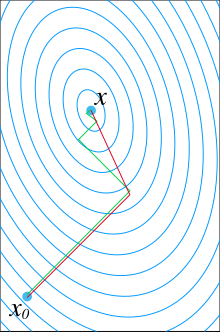
A comparison of the convergence ofgradient descent with optimal step size (in green) and conjugate gradient (in red) for minimizing a quadratic function associated with a given linear system. Conjugate gradient, assuming exact arithmetics, converges in at most n steps where n is the size of the matrix of the system (here n=2).

In mathematics, the conjugate gradient method is an algorithm for the numerical solution of particular systems of linear equations, namely those whose matrix issymmetric and positive-definite. The conjugate gradient method is an iterative method, so it can be applied to sparse systems that are too large to be handled by direct methods such as the Cholesky decomposition. Such systems often arise when numerically solvingpartial differential equations.
The conjugate gradient method can also be used to solve unconstrained optimizationproblems such as energy minimization.
The biconjugate gradient method provides a generalization to non-symmetric matrices. Various nonlinear conjugate gradient methods seek minima of nonlinear equations.

Successive over-relaxation

Successive over-relaxation

From Wikipedia, the free encyclopedia
In numerical linear algebra, the method of successive over-relaxation (SOR) is a variant of the Gauss–Seidel method for solving alinear system of equations, resulting in faster convergence. A similar method can be used for any slowly converging iterative process. It was devised simultaneously by David M. Young and by H. Frankel in 1950 for the purpose of automatically solving linear systems on digital computers. Over-relaxation methods had been used before the work of Young and Frankel. For instance, the method of Lewis Fry Richardson, and the methods developed by R. V. Southwell. However, these methods were designed for computation by human calculators, and they required some expertise to ensure convergence to the solution which made them inapplicable for programming on digital computers. These aspects are discussed in the thesis of David M. Young.[1]

Gauss–Seidel method

Gauss–Seidel method

From Wikipedia, the free encyclopedia
In numerical linear algebra, the Gauss–Seidel method, also known as the Liebmann method or the method of successive displacement, is an iterative method used to solve a linear system of equations. It is named after the German mathematicians Carl Friedrich Gauss and Philipp Ludwig von Seidel, and is similar to the Jacobi method. Though it can be applied to any matrix with non-zero elements on the diagonals, convergence is guaranteed if the matrix is either diagonally dominant, or symmetric and positive definite.