matrix – Ware

Lanczos algorithm

From Wikipedia, the free encyclopedia

The Lanczos algorithm is an iterative algorithm invented by Cornelius Lanczos that is an adaptation of power methods to findeigenvalues and eigenvectors of a square matrix or the singular value decomposition of a rectangular matrix. It is particularly useful for finding decompositions of very large sparse matrices. In Latent Semantic Indexing, for instance, matrices relating millions of documents to hundreds of thousands of terms must be reduced to singular-value form.

Peter Montgomery published in 1995 an algorithm, based on the Lanczos algorithm, for finding elements of the nullspace of a large sparse matrix over GF(2); since the set of people interested in large sparse matrices over finite fields and the set of people interested in large eigenvalue problems scarcely overlap, this is often also called the block Lanczos algorithm without causing unreasonable confusion. See Block Lanczos algorithm for nullspace of a matrix over a finite field.

http://en.wikipedia.org/wiki/Lanczos_algorithm

Complexity of Matrix Inversion

What is the computational complexity of inverting an nxn matrix? (In 
general, not special cases such as a triangular matrix.)

Gaussian Elimination leads to O(n^3) complexity. The usual way to 
count operations is to count one for each "division" (by a pivot) and 
one for each "multiply-subtract" when you eliminate an entry.

Here's one way of arriving at the O(n^3) result:

   At the beginning, when the first row has length n, it takes n 
   operations to zero out any entry in the first column (one division, 
   and n-1 multiply-subtracts to find the new entries along the row 
   containing that entry. To get the first column of zeroes therefore 
   takes n(n-1) operations.

   In the next column, we need (n-1)(n-2) operations to get the second 
   column zeroed out.

   In the third column, we need (n-2)(n-3) operations.

   The sum of all of these operations is:

         n            n         n      n(n+1)(2n+1)   n(n+1)
        SUM i(i-1) = SUM i^2 - SUM i = ------------ - ------
        i=1          i=1       i=1           6           2

   which goes as O(n^3). To finish the operation count for Gaussian 
   Elimination, you'll need to tally up the operations for the process 
   of back-substitution (you can check that this doesn't affect the 
   leading order of n^3).

You might think that the O(n^3) complexity is optimal, but in fact 
there exists a method (Strassen's method) that requires only 
O(n^log_2(7)) = O(n^2.807...) operations for a completely general 
matrix. Of course, there is a constant C in front of the n^2.807. This 
constant is not small (between 4 and 5), and the programming of 
Strassen's algorithm is so awkward, that often Gaussian Elimination is 
still the preferred method.

Even Strassen's method is not optimal. I believe that the current 
record stands at O(n^2.376), thanks to Don Coppersmith and Shmuel 
Winograd. Here is a Web page that discusses these methods:

   Fast Parallel Matrix Multiplication - Strategies for Practical 
   Hybrid Algorithms - Erik Ehrling
http://www.f.kth.se/~f95-eeh/exjobb/background.html   

These methods exploit the close relation between matrix inversion and 
matrix multiplication (which is also an O(n^3) task at first glance). 

I hope this helps! 

- Doctor Douglas, The Math Forum
http://mathforum.org/dr.math/

Complexity of Matrix Inversion

What is the computational complexity of inverting an nxn matrix? (In 
general, not special cases such as a triangular matrix.)

Gaussian Elimination leads to O(n^3) complexity. The usual way to 
count operations is to count one for each "division" (by a pivot) and 
one for each "multiply-subtract" when you eliminate an entry.

Here's one way of arriving at the O(n^3) result:

   At the beginning, when the first row has length n, it takes n 
   operations to zero out any entry in the first column (one division, 
   and n-1 multiply-subtracts to find the new entries along the row 
   containing that entry. To get the first column of zeroes therefore 
   takes n(n-1) operations.

   In the next column, we need (n-1)(n-2) operations to get the second 
   column zeroed out.

   In the third column, we need (n-2)(n-3) operations.

   The sum of all of these operations is:

         n            n         n      n(n+1)(2n+1)   n(n+1)
        SUM i(i-1) = SUM i^2 - SUM i = ------------ - ------
        i=1          i=1       i=1           6           2

   which goes as O(n^3). To finish the operation count for Gaussian 
   Elimination, you'll need to tally up the operations for the process 
   of back-substitution (you can check that this doesn't affect the 
   leading order of n^3).

You might think that the O(n^3) complexity is optimal, but in fact 
there exists a method (Strassen's method) that requires only 
O(n^log_2(7)) = O(n^2.807...) operations for a completely general 
matrix. Of course, there is a constant C in front of the n^2.807. This 
constant is not small (between 4 and 5), and the programming of 
Strassen's algorithm is so awkward, that often Gaussian Elimination is 
still the preferred method.

Even Strassen's method is not optimal. I believe that the current 
record stands at O(n^2.376), thanks to Don Coppersmith and Shmuel 
Winograd. Here is a Web page that discusses these methods:

   Fast Parallel Matrix Multiplication - Strategies for Practical 
   Hybrid Algorithms - Erik Ehrling
http://www.f.kth.se/~f95-eeh/exjobb/background.html   

These methods exploit the close relation between matrix inversion and 
matrix multiplication (which is also an O(n^3) task at first glance). 

I hope this helps! 

- Doctor Douglas, The Math Forum
http://mathforum.org/dr.math/

Rotation matrix

From Wikipedia, the free encyclopedia

In linear algebra, a rotation matrix is a matrix that is used to perform a rotation in Euclidean space. For example the matrix

$R = begin{bmatrix} cos theta & -sin theta \ sin theta & cos theta \ end{bmatrix}$

rotates points in the xy–Cartesian plane counterclockwise through an angle θ about the origin of the Cartesian coordinate system. To perform the rotation, the position of each point must be represented by a column vector v, containing the coordinates of the point. A rotated vector is obtained by using the matrix multiplication Rv (see below for details).

In two and three dimensions, rotation matrices are among the simplest algebraic descriptions of rotations, and are used extensively for computations in geometry, physics, and computer graphics. Though most applications involve rotations in two or three dimensions, rotation matrices can be defined for n-dimensional space.

Rotation matrices are always square, with real entries. Algebraically, a rotation matrix in n-dimensions is a n × n special orthogonal matrix, that is an orthogonal matrix whose determinant is 1:

$R^{T} = R^{-1}, det R = 1,$ .

The set of all rotation matrices forms a group, known as the rotation group or the special orthogonal group. It is a subset of the orthogonal group, which includes reflections and consists of all orthogonal matrices with determinant 1 or -1, and of the special linear group, which includes all volume-preserving transformations and consists of matrices with determinant 1.

http://en.wikipedia.org/wiki/Rotation_matrix

As in two dimensions a matrix can be used to rotate a point (x, y, z) to a point (x′, y′, z′). The matrix used is a 3 × 3 matrix,

$mathbf{A} = begin{pmatrix} a & b & c \ d & e & f \ g & h & i end{pmatrix}$

This is multiplied by a vector representing the point to give the result

$mathbf{A} begin{pmatrix} x \ y \ z end{pmatrix} = begin{pmatrix} a & b & c \ d & e & f \ g & h & i end{pmatrix} begin{pmatrix} x \ y \ z end{pmatrix} = begin{pmatrix} x' \ y' \ z' end{pmatrix}$

The matrix A is a member of the three dimensional special orthogonal group, SO(3), that is it is an orthogonal matrix withdeterminant 1. That it is an orthogonal matrix means that its rows are a set of orthogonal unit vectors (so they are an orthonormal basis) as are its columns, making it easy to spot and check if a matrix is a valid rotation matrix. The determinant must be 1 as if it is -1 (the only other possibility for an orthogonal matrix) then the transformation given by it is a reflection, improper rotation or inversion in a point, i.e. not a rotation.

Matrices are often used for doing transformations, especially when a large number of points are being transformed, as they are a direct representation of the linear operator. Rotations represented in other ways are often converted to matrices before being used. They can be extended to represent rotations and transformations at the same time using Homogeneous coordinates. Transformations in this space are represented by 4 × 4 matrices, which are not rotation matrices but which have a 3 × 3 rotation matrix in the upper left corner.

The main disadvantage of matrices is that they are more expensive to calculate and do calculations with. Also in calculations wherenumerical instability is a concern matrices can be more prone to it, so calculations to restore orthonormality, which are expensive to do for matrices, need to be done more often.

Unitary matrix

From Wikipedia, the free encyclopedia

In mathematics, a unitary matrix is an $ntimes n$ complex matrix U satisfying the condition

$U^{dagger} U = UU^{dagger} = I_n,$

where I_n is the identity matrix in n dimensions and $U^{dagger}$ is the conjugate transpose (also called the Hermitian adjoint) of U. Note this condition says that a matrix U is unitary if and only if it has an inverse which is equal to its conjugate transpose $U^{dagger} ,$

$U^{-1} = U^{dagger} ,;$

A unitary matrix in which all entries are real is an orthogonal matrix. Just as an orthogonal matrix G preserves the (real) inner productof two real vectors,

$langle Gx, Gy rangle = langle x, y rangle$

so also a unitary matrix U satisfies

$langle Ux, Uy rangle = langle x, y rangle$

for all complex vectors x and y, where $langlecdot,cdotrangle$ stands now for the standard inner product on $mathbb{C}^n$ .

If $U ,$ is an n by n matrix then the following are all equivalent conditions:

$U ,$ is unitary
$U^{dagger} ,$ is unitary
the columns of $U ,$ form an orthonormal basis of $mathbb{C}^n$ with respect to this inner product
the rows of $U ,$ form an orthonormal basis of $mathbb{C}^n$ with respect to this inner product
$U ,$ is an isometry with respect to the norm from this inner product
$U ,$ is a normal matrix with eigenvalues lying on the unit circle.

http://en.wikipedia.org/wiki/Unitary_matrix

Normal matrix

From Wikipedia, the free encyclopedia

A complex square matrix A is a normal matrix if

$A^*A=AA^*$

where A* is the conjugate transpose of A. That is, a matrix is normal if it commutes with its conjugate transpose.

If A is a real matrix, then A*=A^T; it is normal if A^TA = AA^T.

Normality is a convenient test for diagonalizability: every normal matrix can be converted to a diagonal matrix by a unitary transform, and every matrix which can be made diagonal by a unitary transform is also normal, but finding the desired transform requires much more work than simply testing to see whether the matrix is normal.

The concept of normal matrices can be extended to normal operators on infinite dimensional Hilbert spaces and to normal elements in C*-algebras. As in the matrix case, normality means commutativity is preserved, to the extent possible, in the noncommutative setting. This makes normal operators, and normal elements of C*-algebras, more amenable to analysis.

http://en.wikipedia.org/wiki/Normal_matrix

Hermitian matrix

From Wikipedia, the free encyclopedia

In mathematics, a Hermitian matrix (or self-adjoint matrix) is a square matrix with complex entries that is equal to its ownconjugate transpose – that is, the element in the i-th row and j-th column is equal to the complex conjugate of the element in the j-th row and i-th column, for all indices i and j:

$a_{i,j} = overline{a_{j,i}},.$

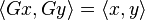
If the conjugate transpose of a matrix A is denoted by $A^dagger$ , then the Hermitian property can be written concisely as

$A = A^dagger,.$

Hermitian matrices can be understood as the complex extension of real symmetric matrices.

Hermitian matrices are named after Charles Hermite, who demonstrated in 1855 that matrices of this form share a property with real symmetric matrices of having eigenvalues always real.

http://en.wikipedia.org/wiki/Hermitian_matrix

Spectral radius

From Wikipedia, the free encyclopedia

In mathematics, the spectral radius of a matrix or a bounded linear operator is the supremum among the absolute values of the elements in its spectrum, which is sometimes denoted by ρ(·).

http://en.wikipedia.org/wiki/Spectral_radius

Inverse iteration

From Wikipedia, the free encyclopedia

In numerical analysis, inverse iteration is an iterative eigenvalue algorithm. It allows to find an approximate eigenvector when an approximation to a corresponding eigenvalue is already known. The method is conceptually similar to the power method and is also known as the inverse power method.

http://en.wikipedia.org/wiki/Inverse_iteration

Rayleigh quotient iteration

From Wikipedia, the free encyclopedia

Rayleigh quotient iteration is an eigenvalue algorithm which extends the idea of the inverse iteration by using the Rayleigh quotient to obtain increasingly accurate eigenvalue estimates.

Rayleigh quotient iteration is an iterative method, that is, it must be repeated until it converges to an answer (this is true for all eigenvalue algorithms). Fortunately, very rapid convergence is guaranteed and no more than a few iterations are needed in practice. The Rayleigh quotient iteration algorithm converges cubically, given an initial vector that is sufficiently close to an eigenvector of thematrix that is being analyzed.

http://en.wikipedia.org/wiki/Rayleigh_quotient_iteration